This breakdown comes out of the same pipeline I use for my UFC prediction models: a big PostgreSQL feature store, opponent-adjusted stats, time decay, and a ton of Bayesian smoothing.
I'm not claiming to be an official analyst or anything like that. This is just my best effort to point the math at the UFC and say:
"Okay, which fighters look genuinely weird for their weight class right now?"
If something seems off, or you've got ideas for better thresholds or features, feel free to roast or suggest improvements in the comments. I'm iterating this all the time.
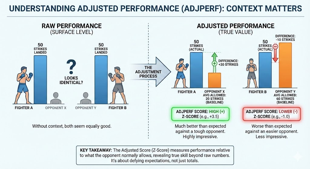
What Is Adjusted Performance (AdjPerf)?
Everything in here is driven by adjusted performance, or adjperf.
At a high level, adjperf answers:
"How did this fighter perform compared to what their opponent normally allows, within their weight class?"
Plain English version:
- Every opponent has a history of what they usually allow:
- How many sig strikes per minute they eat
- How many takedowns they give up
- How often they get subbed, dropped, controlled, etc.
- In a given fight, we compare what our fighter did vs that opponent's "allowed" baseline.
- We normalize that difference using a robust measure of spread (MAD, not vanilla standard deviation).
- We get a z-score inside that weight class:
- 0 = perfectly average for that matchup
- +1 to +2 = clearly above average
- +3+ = extreme
- Scores are clipped to ±7 so they don't blow up the model
High adjperf = you did something to that opponent that other fighters in your weight class usually cannot do.
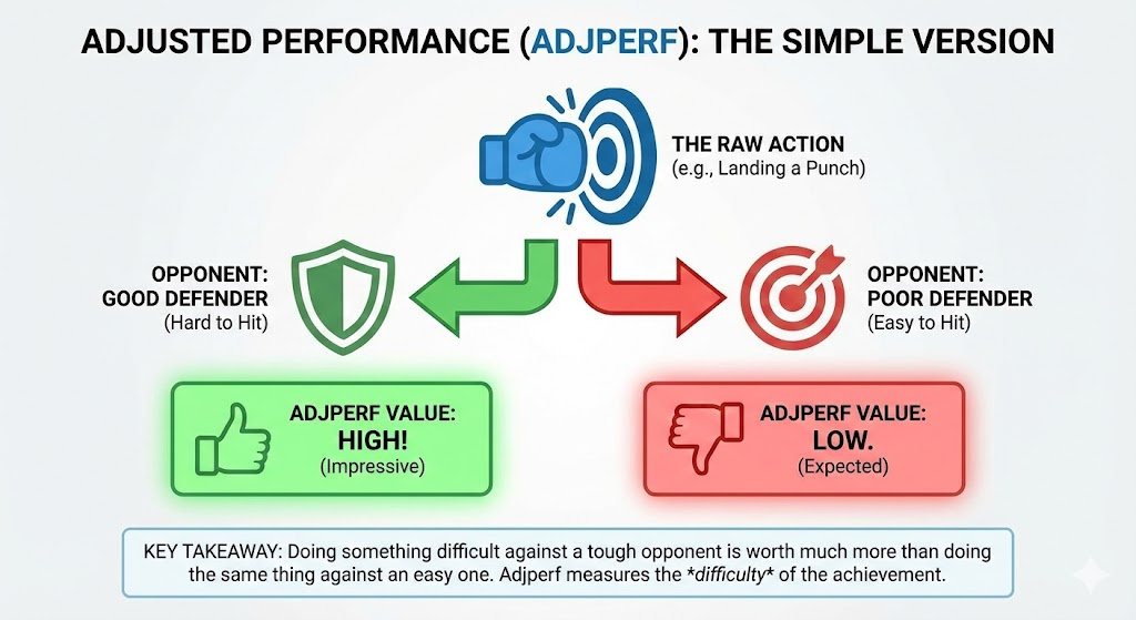
Simplified overview of how adjperf works
How AdjPerf Actually Works (Nerd Corner)
If you like the guts, here's the rough shape of the math.
For a given stat (say, takedowns per minute), we compute:
adjperf = clip((observed − μ_shrunk) / MAD_shrunk, −7, +7)Where:
- Observed = the fighter's stat in that fight (already on a canonical per-minute / rate scale).
- Opponent history (allowed):
- We look at what that opponent's past opponents have done against them.
- Compute an opponent-level mean and MAD of "allowed" values, with optional time-decay so recent fights matter more.
- Weight-class prior:
- We have a weight-class mean and MAD for that stat (flyweight, bantamweight, etc.).
- Bayesian shrinkage:
- We blend opponent history and weight-class prior:
wherew = n / (n + K)nis effective sample size (Kish-adjusted under decay). - Small
n→ we lean more on the weight-class prior. - Large
n→ we trust the opponent-specific history. - That gives:
μ_shrunk = w_mean · μ_opp + (1 − w_mean) · μ_wc
MAD_shrunk = max(w_mad · MAD_opp + (1 − w_mad) · MAD_wc, MAD_floor)
- We blend opponent history and weight-class prior:
- Clipping:
- Final z-scores are clipped to ±7 in the feature store so extreme fights don't dominate training.
So adjperf is:
- Opponent-aware
- Weight-class-aware
- Time-aware (via decay)
- And robust (using MAD + shrinkage + clipping)
It's not just "he had a big fight once" — it's "given who he fought, in this weight class, how far off the expected distribution was that performance?"
Detailed technical breakdown of the adjperf calculation pipeline
For this article, I'm looking at time-decayed adjperf so we're capturing current form, not ancient history.
How Fighters Made This List
To show up here, a fighter had to:
- Be a clear adjperf outlier in their weight class
- Their most recent time-decayed adjperf for that stat is way out on the tail.
- We're talking "this would make a data scientist raise an eyebrow" levels.
- Have raw stats that tell the same story
- Attempts, land rates, per-minute numbers from actual fight logs line up with the adjperf narrative.
Adjperf itself is already the primary signal — it's built to be stable and opponent-aware. The raw stats you see below are there to make the story readable and to give you something concrete to sanity-check against (and yell at me about if you disagree).
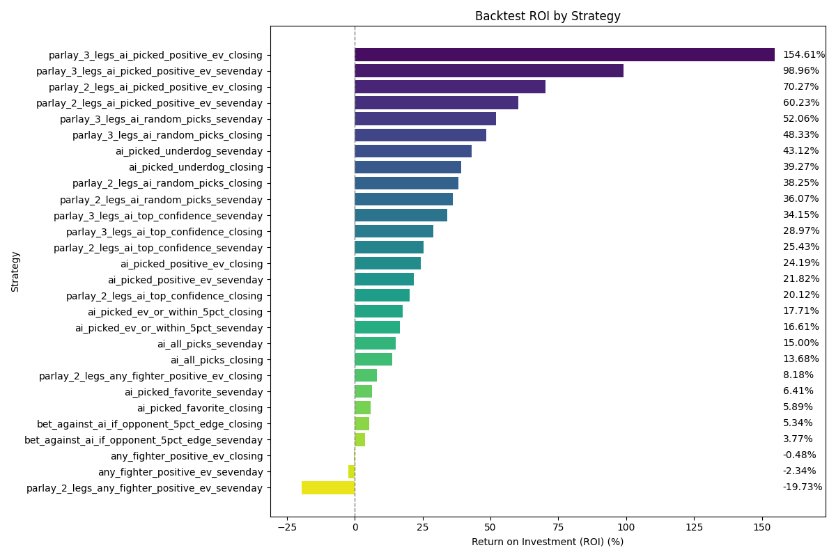
The 13 Most Extreme Statistical Outliers of 2025
1. Valter Walker – Heavyweight Submission Goblin
Stat: Submission attempts per minute
Most Recent AdjPerf: +53.60 (pre-clipping)
Weight Class: Heavyweight
UFC Fights: 5
Most Recent Fight: 2025-10-25
Heavyweight is supposed to be overhands and brain cells leaving the building. Walker is out here playing "lightweight jiu-jitsu specialist" instead.
Raw rate: 0.561 submission attempts per minute
- Attempts by fight: 1, 1, 1, 1, 0
- Fight times: 1.4, 0.9, 1.3, 4.9, 15.0 minutes
Against heavyweights who usually don't even give up many sub attempts, this is wild. Adjperf is basically saying:
"Relative to what heavyweights normally allow, this guy is constantly hunting submissions in a division that does not do that."
He's a genuine grappling outlier at heavyweight.
2. Anshul Jubli – Lightweight Touch-of-Death Candidate
Stat: KO efficiency (KOs per sig strike landed)
Most Recent AdjPerf: +31.73
Weight Class: Lightweight
UFC Fights: 3
Most Recent Fight: 2025-02-08
Most lightweights need accumulation. Jubli just needs the right connection.
- 1 KO from 141 sig strikes total (0.7% overall)
- In the KO fight: 1 KO from 38 sig strikes (~2.6% in that bout)
Adjperf adjusts for who he knocked out and how hard they are to finish. The model is essentially screaming "this wasn't just some glass-chin mercy-stoppage."
Small sample size, yes. But early data says: when he lands clean, it ends badly for people.
3. Merab Dvalishvili – Takedown Volume Barbarian
Stat: Takedown attempts per minute
Most Recent AdjPerf: +6.53
Weight Class: Bantamweight
UFC Fights: 17
Most Recent Fight: 2025-12-06
Most fighters shoot to mix things up. Merab shoots as a lifestyle.
- 117 takedown attempts over his UFC run
- 1.085 attempts per minute
- Recent 25-minute fights: 29, 37, 30, 15 attempts
Adjperf compares that volume to what his opponents usually allow. Elite defensive wrestlers who normally see ~0.3 attempts/min are getting bombarded at over 1 attempt/min.
Even if you're sitting on elite takedown defense, math starts to cave in when someone chains 30+ attempts on you. You defend, you get up, you defend again, forever.
4. Jailton Almeida – Heavyweight Takedown Factory
Stat: Takedowns landed per minute
Most Recent AdjPerf: +11.37
Weight Class: Heavyweight
UFC Fights: 10
Most Recent Fight: 2025-10-25
First he gets you down. Then you stay there. The first part is this section.
- 34 takedowns total
- 0.514 takedowns per minute
- Examples:
- 7 takedowns in a 15-minute fight
- 6 in a 25-minute fight
Against heavyweights who normally do not get taken down much, that's a big departure from the baseline.
Adjperf is calling out that he's consistently converting takedowns at a rate his opponents do not usually allow — and that's the on-ramp to his entire submission game.
5. Hamdy Abdelwahab – "If I Shoot, You Sit"
Stat: Takedown accuracy
Most Recent AdjPerf: +26.68
Weight Class: Heavyweight
UFC Fights: 4
Most Recent Fight: 2025-10-25
Hamdy's story isn't volume; it's precision.
- 13 takedowns on 20 attempts (65.0% accuracy)
- Most recent fight: 9/14 (64.3%)
Heavyweights are usually pretty good at just being big and hard to drag down. Adjusted for opponent TDD, +26.68 is the model saying "these guys don't normally get hit with this many clean entries."
It's still an early sample, but the technique and efficiency are tracking as outliers.
6. Kyoji Horiguchi – Flyweight Knockdown Glitch
Stat: Knockdowns per minute
Most Recent AdjPerf (pre-clip): +945.00
Weight Class: Flyweight
UFC Fights: 9
Most Recent Fight: 2025-11-22
This is the single craziest value in the whole system before clipping. Here's why it explodes:
- Knockdowns at 125 are extremely rare.
- That makes the weight-class MAD for KD/min tiny.
- When someone genuinely overperforms there, the un-clipped z-score goes to the moon.
In practice:
- 6 knockdowns in 9 UFC fights
- Career KD rate: 0.053 per minute
- 2025 fight: 2 knockdowns in 12.3 minutes (0.163 KD/min)
In the live feature store, this gets clipped at +7 for sanity, but the underlying signal is still: for flyweight, this guy's knockdown production is absurd.
And he's not just raw power — it's timing, entries, and shot selection built on years of striking experience.
7. Joshua Van – Endless Output at Flyweight
Stat: Significant strikes landed per minute
Most Recent AdjPerf: +5.30
Weight Class: Flyweight
UFC Fights: 10
Most Recent Fight: 2025-12-06
Van fights like the slider for "pace" is stuck all the way to the right.
- 1,099 sig strikes total
- 8.354 sig strikes per minute
- Recent fights: 204 strikes (15 min), 125 strikes (14 min), 165 strikes (15 min)
Adjperf compares that to what his opponents usually allow and flags him as a clear outlier. These are fast, defensively sharp flyweights, and he's still landing at a pace most guys can't match for a round, never mind three.
His win condition is simple: survive his pace or break.
8. Ciryl Gane – Overall Accuracy Cheat Code
Stat: Overall strike accuracy
Most Recent AdjPerf: +2.93
Weight Class: Heavyweight
UFC Fights: 13
Most Recent Fight: 2025-10-25
Gane is what happens when a heavyweight actually cares about clean shot selection.
- 929 of 1,507 total strikes landed (61.6% accuracy)
- Last three fights: 75.0%, 70.5%, 69.9% total accuracy
Adjperf is factoring in the fact that his opponents typically don't get lit up at these percentages. For heavyweight, where a lot of guys swing big and miss a lot, this level of sustained efficiency is unusual.
Volume isn't crazy; the quality of each attempt is.
9. Ciryl Gane – Distance Sniper
Stat: Distance strike accuracy
Most Recent AdjPerf: +4.04
Weight Class: Heavyweight
UFC Fights: 13
Most Recent Fight: 2025-10-25
If #8 is the macro view, this is his true specialty: long-range work.
- 837 of 1,394 distance strikes landed (60.0% distance accuracy)
- Recent fights at distance: 75.0%, 70.2%, 69.1%
Most heavyweights are happy to crack 40–45% at distance against top guys. Gane is living in the 60–70% range.
Adjperf is saying: even after adjusting for how little these opponents normally let others hit them at range, Gane is still an outlier.
He appears twice on this list because his game is systematically efficient, not just one big performance skating the numbers.
10. Payton Talbott – Headshot Specialist at Bantamweight
Stat: Head strike accuracy
Most Recent AdjPerf: +2.91
Weight Class: Bantamweight
UFC Fights: 6
Most Recent Fight: 2025-12-06
Talbott doesn't just land; he finds the head consistently.
- 262 of 498 head strikes landed (52.6% head accuracy)
- Most recent fight: 89 of 167 to the head (53.3%)
Bantamweight is full of guys with great head movement, footwork, and defense. Maintaining 50%+ head accuracy fight after fight against that kind of opposition is rare.
Adjperf incorporates opponent defensive quality and still puts him clearly above the curve. High volume plus high precision to the most important scoring target is exactly what judges (and knockouts) like.
11. Jean Matsumoto – Leg Kick Merchant
Stat: Leg strike share (% of total strikes to the legs)
Most Recent AdjPerf: +3.17
Weight Class: Bantamweight
UFC Fights: 4
Most Recent Fight: 2025-08-09
Matsumoto doesn't just "use" leg kicks; he builds entire days around them.
Per fight:
- Leg kicks: 19, 25, 21, 8
- Total sig strikes: 95, 77, 89, 19
- Leg kick share: 20.0%, 32.5%, 23.6%, 42.1%
Adjperf compares his leg-kick focus to what opponents usually face and flags him as a specialization outlier. He's still going hard to the legs even against guys who historically defend or avoid them well.
This is classic Dutch kickboxing logic applied in MMA: attack the base until the opponent can't move or plant properly late in the fight.
12. Kyoji Horiguchi – Top-Game Controller at Flyweight
Stat: Ground strike percentage (% of sig strikes from ground positions)
Most Recent AdjPerf: +5.79
Weight Class: Flyweight
UFC Fights: 9
Most Recent Fight: 2025-11-22
Same guy as the knockdown glitch, now on the grappling axis.
- 2025 fight: 24 of 49 sig strikes from the ground (49.0%)
Adjperf is adjusting for the fact that his opponents typically keep fights standing against most other people. Horiguchi is dragging them into long stretches of top control and doing meaningful work from there.
At flyweight, where scrambling and standups are usually constant, being able to actually hold people down and build offense is a skill that really stands out in the data.
He's on this list twice because he's extreme in two totally different ways: dropping people and riding them.
13. Jailton Almeida – Control Time Tyrant
Stat: Control time per minute
Most Recent AdjPerf: +10.12
Weight Class: Heavyweight
UFC Fights: 10
Most Recent Fight: 2025-10-25
We covered his takedowns already. Control time is the second half of the nightmare.
- 3,759 total seconds of control
- 49.775 seconds of control per minute (out of 60)
- Recent examples:
- 647 seconds of control in a 15-minute fight (~10.8 minutes)
- 1,270 seconds in a 25-minute fight (~21.2 minutes)
Adjperf measures this against how much control his opponents usually give up. For most heavyweights, being stuck under someone that long is unusual; for Almeida, it's just the pattern.
He shows up twice because in the data he's basically:
- Getting you down at an above-normal rate, and
- Keeping you there at an above-normal rate.
From a modeling perspective, that's a very clear and very stable identity.
Quick Glossary
Z-score (σ)
How many robust standard deviations (via MAD) above or below the weight-class average a performance is:
- +3.0σ and up: extreme outlier
- +2.0σ to +3.0σ: elite
- +1.5σ to +2.0σ: very strong
- +1.0σ+: clearly above average
Adjusted Performance (adjperf)
Opponent-adjusted, weight-class-adjusted, time-decayed z-score:
- Centers on what that opponent typically allows (with shrinkage toward weight-class norms).
- Uses MAD instead of standard deviation for robustness.
- Clipped to ±7 to keep the model stable.
Time-decayed average (dec_avg)
A rolling average where recent fights get more weight. This gives you "who this fighter is now" instead of letting old fights dominate.
Weight-class comparison
All adjperf calculations are done inside the fighter's own weight class:
- Flyweights are compared to other flyweights.
- Heavyweights to heavyweights.
- No cross-weight-class nonsense.
Validation Philosophy
For the model, adjperf is the primary signal. It's designed to already reflect:
- Opponent quality
- Weight-class context
- Sample size and volatility
- Recency
For this article, I layered on a simple sanity check:
- Adjperf says "this is an outlier."
- I check that the raw fight stats (attempts, land rates, per-minute values) tell a story that matches what the metric is flagging.
If adjperf had someone barely above average and the write-up would be pure cope, they didn't make the list. If adjperf had someone pinned near the ceiling but the fight log clearly didn't fit the narrative, I left them out as well.
This is my best attempt to blend a pretty serious statistical pipeline with writeups that still connect to what you see on tape. If you think I missed someone, or you've got ideas on better stats to adjperf-ify next, drop it in the comments — I'm always tuning this.